Monthly Archives

5 Articles

Posted by Anna Brandt on

Tools in the Layout tab

Release 1.10.

The layout tab has two more tools, which we did not mention in our last post. They are especially useful for correcting the layout and save you from annoying detail work.
The first one corrects the Reading Order. If one or more text regions are selected, this tool automatically arranges the child shapes, in this case the lines and baselines, according to their position in the coordinate system of the page. So the reading order starts at the top left and continues counting from there to the bottom right.  In the example below, a TR was split but the RO of the marginal notes got mixed up. This tool saves you now from renaming each BL individually.

The second tool (“assign child shapes”) helps to assign the BL to the correct TR. This can happen when cutting text regions or baselines that run through multiple TRs. Each BL then has to be marked in the layout tab and moved to the correct TR. For assigning them automatically to the corresponding TR you just select the TR where the BLs belong to and start the tool.

Posted by Dirk Alvermann on

“between the lines” – Handling of inserts

At least as often as deletions or blackenings, there are overwritings or inserted text passages written between the lines. It is useful in two aspects to clarify at the beginning of a project how these cases should be handled.

In this simple example you can see how we handle such cases.

Since we include erasures and blackening in both layout and text, it is a logical step to treat overwrites and insertions in the same way. Usually, such passages are already provided with separate baselines during the automatic layout analysis. Every now and then you have to make corrections. In any case, each insertion is treated by us as a separate line and is also taken into account accordingly in the reading order.

Under no circumstances should you transcribe overwrites or insertions above the line instead of deletions. This would falsify the training material, even though the presentation of the text would of course be more pleasing to the human eye.

Posted by Dirk Alvermann on

Treatment of erasures and blackenings

HTR models treat erased text the same as any other. They know no difference and therefore always provide a reading result. In fact, they are amazingly good at it, and read useful content even where a transcriber would have given up long ago.

The simple example shows an erased text that is still legible to the human eye and which the HTR model has read almost without error.

Because we have already seen this ability of the HTR models in other projects, we decided from the beginning to transcribe as much of the erased and blacked out text as possible in order to use the potential of the HTR. The corresponding passages are simply tagged as text-style “strike through” in the text and thus remain recognizable for possible internal search operations.

If you don’t want to make this effort, you have the possibility to intervene in the layout at the corresponding text passages that contain erasures or blackenings and, for example, delete the baselines or shorten them accordingly. Then the HTR does not “see” such passages and cannot recognize them. But this is not less complex than the way we have chosen.

Under no circumstances should you work on erasures with the “popular” expression “[…]”. The transcribers know what the deletion sign means, but the HTR learns something completely wrong here, when many such passages come into training.

Posted by Elisabeth Heigl on

Test samples – the impartial alternative

If a project concept does not allow the strategic planning and organization of test sets, there is a simple alternative: automatically generated samples. Samples are also a valuable addition to the manually created test sets, because here it is the machine that decides which material is included in the test and which is not. Transkribus can select individual lines from a set of pages that you have previously provided. So it’s a more or less random selection. This is worthwhile for projects that have a lot of material at their disposal – including ours.

We use samples as a cross-check to our manually created test sets and because samples are comparable to the statistical methods of random sampling, which the DFG also recommends in its rules of practice for testing the quality of OCR.

Because HTR – unlike OCR – is line-based, we modify the DFG’s recommendation somewhat. I will explain this with an example: For our model Spruchakten_M-3K, a check should be carried out on the reading accuracy achieved. For this purpose we created a sample, exclusively from untrained material of the whole period for which the model works (1583-1627). To do this, we selected every 20th page from the entire data set, obtainimg a subset of 600 pages. It represents approximately 3.7% of the total 16,500 pages of material available for this period.  All this is done on your own network drive. After uploading this subset to Transkribus and processing it with the CITlab Advanced LA (16.747 lines were detected), we let Transkribus create a sample from it. It contains 900 randomly selected lines. This is about 5% of the subset. This sample was now provided with GT and used as a test set to check the model.

And this is how it works in practice: The “Sample Compare” function is called up in the “Tools” menu. Select your subset in the collection and add it to the sample set pressing the “add to sample” button. Then specify the number of lines Transkribus should select from the subset. Here you should select at least as many lines as there are pages in the subset, so that each page has one test line.

In our case, we decided to use a factor of 1.5 just to be sure. The program now selects the lines independently and compiles a sample from them, which is saved as a new document. This document does not contain any pages, but only lines. These must now be transcribed as usual to create GT. Afterwards any model can be tested on this test set using the Compare function.

Posted by Elisabeth Heigl on

Image resolution

A technical parameter that needs to be uniformly determined at the beginning of the scanning process is the resolution of the digital images, that means how many pixels/dots per inch (dpi) the scanned image should have.

The DFG Code of Practice for Digitisation generally recommends 300 dpi (p. 15). For “text documents with the smallest significant character” of up to 1.5 mm, however, a resolution of 400 dpi can be selected (p. 22). Indeed, in the case of manuscripts – especially concept writings – of the early modern period, the smallest character components can result in different readings and should therefore be as clearly identifiable as possible. We have therefore chosen 400 dpi.

In addition to the advantages for deciphering the scripts, however, the significantly larger storage format of the 400 (around 40,000 KB/img.) compared to the 300 (around 30,000 KB/img.) files must be taken into account and planned for!

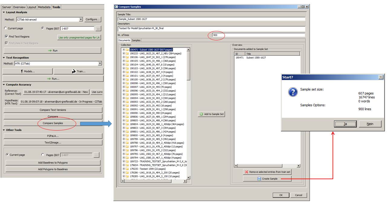
The selected dpi number also has an impact on the process of automatic handwritten text recognition. Different resolutions lead to different results of the layout analysis and the HTR. To verify this thesis, we have selected three pages from a speech file of 1618, scanned them in 150, 200, 300 and 400 dpi each, processed all pages in transcript and determined the following CERs:

Seite/dpi 150 200 300 400
2 3,99 3,5 3,63 3,14
5 2,1 2,37 2,45 2,11
9 6,73 6,81 6,52 6,37

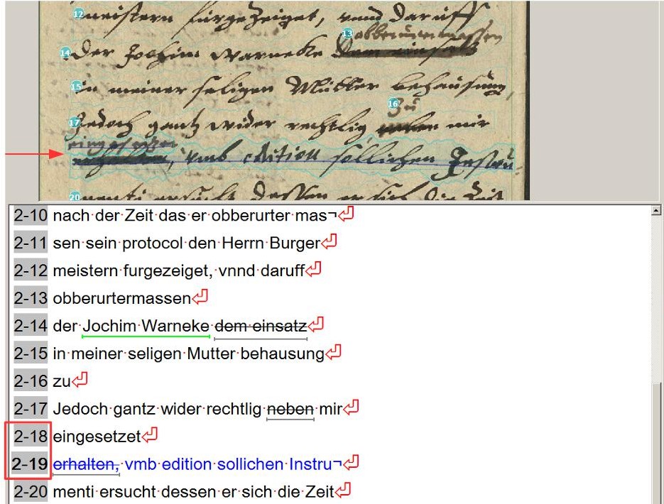
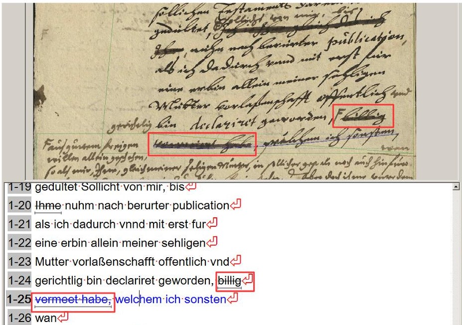
Generally speaking, a lower resolution therefore means a decrease in CERs – though within the range of less than one percent.To be honest, such comparisons of HTR results are somewhat misleading. The very basis of the HTR – the layout analysis – leads to latently different results at different resolutions, which in turn influences the HTR results (apparently cruder analyses achieve worse HTR results) but also the GT production itself (e.g. with cut-off words).

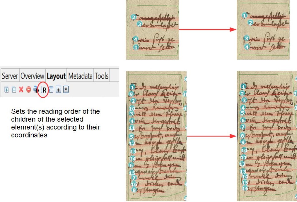
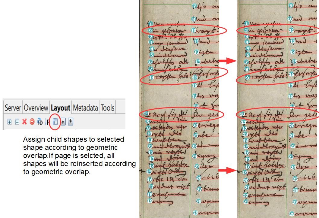
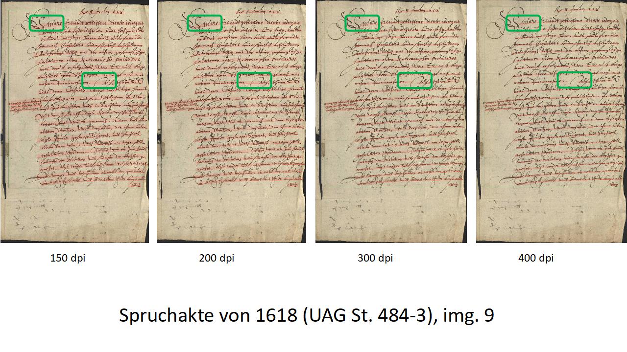
In our example you see the same image in different resolutions. The result of the CITlab Advanced LA changes as the resolution increases. The initial “V” of the first line is no longer recognized at higher resolution, while line 10 is increasingly “torn apart” at higher resolution. With increasing resolution, the LA becomes more sensitive – this can have advantages and disadvantages at the same time.

It is therefore important to have a uniform dpi number for the entire project so that the average CER values and the entire statistical material can be reliably evaluated.