Yearly Archives

34 Articles

Posted by Dirk Alvermann on

HTR+ versus Pylaia

Version 1.12.0

As you have probably noticed, since last summer there is a second recognition engine available in Transkribus besides HTR+ – PyLaia. (link)

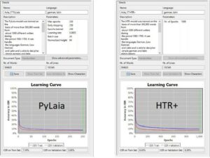
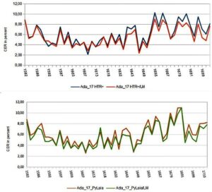
We have been experimenting with PyLaia models in the last weeks and would like to document our first impressions and experiences about the different aspects of HTR+ and PyLaia. First of all: considering the economic point of view, PyLaia is definitely a little bit cheaper than HTR+, as you can see on the price list of the Read Coop. Does cheaper also mean worse? – Definitely not! In terms of accuracy rate PyLaia can easily compete with HTR+. It is often slightly better. The following graphic compares an HTR+ and a PyLaia model trained with identical ground truth (approx. 600,000 words) under the same conditions (from the scratch). The performance with and without the Language Model is compared.

Perhaps the most notable difference is that the results of PyLaia models cannot be improved as much by using a Language Model as is the case with HTR+. This is not necessarily a disadvantage, but rather indicates a high basic reliability of these models. In other words: PyLaia does not necessarily need a Language Model to achieve very good results.

There is also an area where PyLaia performs worse than HTR+. PyLaia has more difficulties to read “curved” lines correctly. For vertical text lines the result is even worse.

In training PyLaia is a bit slower than HTR+, which means that the training takes longer. On the other hand, PyLaia is much faster in “acceleration”. It needs relatively few training epochs or iterations to achieve good results. You can compare this quite well with the two learning curves.

Our observations are of course not exhaustive. So far they only refer to generic models that have been trained with a high level of ground truth. Overall we have the impression that PyLaia can fully exploit its advantages with such large generic models.

Posted by Dirk Alvermann on

How to train PyLaia models

Release 1.12.0

Since version 1.12.0 it is possible to train PyLaia models in Transkribus besides the proven HTR+ models. We have gained some experience with this in the last months and are quite impressed by the performance of the models.

PyLaia models can be trained like HTR or HTR+ models using the usual training tool. But there are some differences.

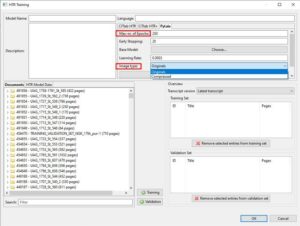
Like a normal HTR+ model you have to enter the name of the model, a description and the languages the model can be used for. Unlike the training of HTR+ models, the number of iterations (epochs) is limited to 250. This is sufficient in our experience. You can also train PyLaia models with base models, i.e. you can design longer training series that are based on each other. In contrast to the usual training, PyLaia has an “Early Stopping” setting. It determines when the training can be stopped, if a good result is achieved. At the beginning of your training attempts you should always set this value to the same number of iterations as you have chosen for the whole training. So if you train with 250 epochs, the setting for “Early Stopping” should be the same. Otherwise you risk that the training will be stopped too early.

The most important difference is that in PyLaia Training you can choose whether you want to train with the original images or with compressed images. Our recommendation is: train with compressed images. The PyLaia training with original images can take weeks in the worst case (with a correspondingly large amount of GT). With compressed images a PyLaia training is finished within hours or days (if you train with about 500.000 words).

Tips & Tools
For more detailed information, especially for setting specific training parameters, we recommend the tutorial by Annemieke Romein and the READ Coop guidelines.

Posted by Dirk Alvermann on

Our first public model for german current (17th century)

Today we proudly present our HTR-model “Acta 17” as a public model.

The model was trained on the base of more than 500,000 words from about a 1000 different writers during the period of 1580-1705. It can handle the languages German, Lower German and Latin and is able to decipher simple german and latin abbreviations. Besides the usual chancellery lettering, the training material also contained a selection of concept writings and printed material of the period.

The entire training material is based on legal texts or court writings from the Responsa of the Greifswald Law Faculty. Validation sets are based on a chronological selection of the years: 1580 – 1705. GT & validation set was produced by Dirk Alvermann, Elisabeth Heigl, Anna Brandt.

Due to some problems with creating a large series of base-model-trainings for HTR+ Models in the last couple of weeks, we decided to launch an HTR+ Model trained from the scratch.

It is accompanied by a PyLaia model, which is based on the same training and validation sets and was also trained without using a base model.

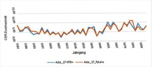
For the validation set we choose pages representing single years of the total set of documents. All together they represent 48 selected years, five pages of each year.

How the models do perform in the several time periods of the validation set, you can check in the comparison below. Both models did run without language model.

Posted by Anna Brandt on

Searching and editing tags

Release 1.11.0

If you tag large amounts of historical text, as we have tried to do with place and person names, you will sooner or later have a problem: the spelling varies a lot – or in other words, the tag values are not identical.
Let’s take the places and a simple example. As “Rosdogk”, “Rosstok” or “Rosdock” the same place is always referred to – the City of Rostock. To make this recognizable, you use the properties. But if you do this over more than ten thousand pages with hundreds or thousands of places (we set about 15,000 tags for places in our attempt), you easily lose the overview. And besides, tagging takes much longer if you also assign properties.

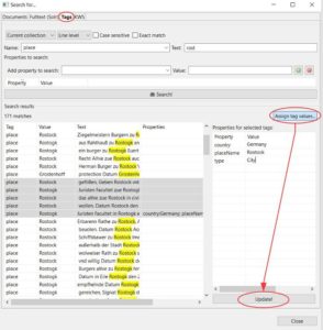
Fortunately, there is an alternative. You can search in the tags, not only in the document you are working on, but in the whole collection. To do this, you just have to select the “binoculars” in the menu, similar to starting a full text search or KWS, only that you now select the submenu “Tags”.

Here you can select the search area (Collection, Document, Page) and also on which level you want to search (Line or Word).Then you have to select the corresponding tag and if you want to limit the search, you have to enter the tagged word. The search results can also be sorted. This way we can quickly find all “Rostocks” in our collection and can enter the desired additional information in the properties, such as the current name, geodata and similar. These “properties” can then be assigned to all selected tagged words. In this way, tagging and enrichment of data can be separated from each other and carried out efficiently.

The same is possible with tags like “Person” or “Abbrev” (where you would put the resolution/expansion in the properties).

Posted by Dirk Alvermann on

textual tagging

Like everything else, tagging can be integrated into your work on very different levels and with different requirements. In Transkribus, a large number of tags are available for a wide range of applications, some of which are described here.

We decided to try it with only two tags, namely “person” and “place”. These tags will later allow systematic access to the corresponding text passages.

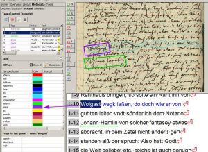
When tagging, Transkribus automatically adopts the term under the cursor as “value” or “label” for the specific case. So if I mark “Wolgast” as in the example below and tag it as “place”, then two important pieces of information are already recorded. The same is true for the name of the person further down.

Transkribus offers the possibility to assign properties to each tagged element, e.g. to display the historical place name in modern spelling or to assign a gnd number to the person’s name. You can also create additional properties, geodata for places etc.

Given the amount of text we process, we have decided not to assign properties to our tags. Only the place names are identified as best as possible. The aim is to be able to display the tag-values separately for people and places next to the respective document when presenting them in the viewer of the Digital Library M-V, thus enabling the user to navigate systematically through the document.

Posted by Anna Brandt on

Tagging in WebUI

For tasks like tagging already transcribed documents, the WebUI, which is especially designed for crowd sourcing projects, is very well suited.

Tagging in the WebUI works slightly different than in the Expert Client. There are different tools and settings.

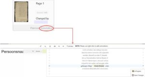
If you have selected your collection and the document in the WebUI and want to tag something, you have to select “Annotation” and not “plain text” for the page you want to edit.  Both modes are similar, except that in Annotation you can additionally tag. To do this, you need to select the words and right-click on them to pick the appropriate tag. Always save when you leave the page, even if you switch to layout mode. The program doesn’t ask you to save the tag as it does in the Expert Client and without saving your tags will be lost.

All tags appear to the left of the text field when you click on the word. The tags set in the Expert Client are also displayed there. The whole annotation mode is still in a beta version at the moment.

Posted by Anna Brandt on

Tagging Tools

Release 1.11.0

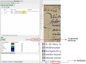
In a previous post we already wrote about our experiences with structure tagging and described the tools that go with it. But for most users (e.g. in edition projects) enriching texts with additional content information is even more important. To add tags to a transcription you can use the tagging tools in the tab “Metadata”/”Textual” in Transkribus.

Here you can see the available tags as well as those that have already been applied to the text of the page. With the Customize button you can create your own tags or add shortcuts to existing tags, just like with structure tagging. The shortcuts allow for easier and faster tagging in the transcript. If you want to do without shortcuts, you have to mark the respective words in the text (not in the image) and select the desired tag with a right click. Of course a word can be tagged several times.

These tags should not be confused with the so-called TextStyles (for example, crossed out or superscript words). They are not accessible below the tags but via the toolbar at the bottom of the text window.

Posted by Dirk Alvermann on

Tagging: what for? – when and why tagging makes sense

Tagging allows – in addition to content indexing by HTR – systematic indexing of the text by the later user. In contrast to an HTR model that does its work independently, tagging has to be done mostly by hand, which means that it requires a lot of effort. Therefore, a realistic effort analysis should be carried out before developing far-reaching plans regarding tagging.

Due to the amount of material processed in our project, we primarily use tagging where it helps us in the practical work on the text. This is the case with structure tagging, where the layout analysis is improved with the help of the tagging and the P2PaLA developed from it, and then of course also with the tagging of textstyles in case of deletions and blackening. This is where tagging is basically used “area-wide” by us. A fixed component of our transcription rules is also the use of the “unclear” tag for passages that cannot be read correctly by the transcriber. In this case, the tag is used more for internal team communication.

For the systematic preparation of texts for which an HTR has already been performed, we are experimenting with the “person” and “place” tags in order to offer systematic indexing, at least in this limited form.

Posted by Elisabeth Heigl on

Compare Samples

Release 1.10.1

As the name suggests, the Compare Samples tool tests the capabilities of an HTR model based on a sample rather than a manually selected test set. We have explained in an earlier post how to create such samples, that they represent an objective alternative to conventional test sets and why they can be created with much less effort.

“Compare Samples” may look like a validation tool, but is actually not one of them. You can use it to validate an HTR model, but Advanced Compare is better suited for this.  The real function of “Sample Compare” is to make predictions about the success of an HTR model on a given material.

You may remember the Model Booster. There you need a suitable HTR model that can serve as a base model for a planned HTR training. With the numerous Public Models available, it is a good idea to first check with “Compare Samples” which model fits to your project.

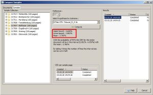
To create such a prediction for a sample, you first have to run the selected HTR models over the entire sample (before that, of course, you have already created the GT for the sample). Then open the Samples tab of the “Compare Samples” tool. This tab lists all samples of your active collection. You select the sample that will be used as the basis for the prediction. Now you can select the model in the middle, whose text version should serve as a reference for the GT. Start “Compute” and you’re done.

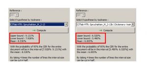
The tool now calculates average values for all lines of the sample with an upper bound, a lower bound and an average value. In the range between upper bound and lower bound you should find the Character Error Rate for 95% of your material at which the selected HTR model is expected to work.  In our example below, between 4,7 and 2,9 %.

This way you can compare as many models for your material as you like. But the tool also allows a few other things. For example, you can easily check how an HTR model with or without language model or dictionary works on your material and if it is worth using one or the other. Of course this is especially useful to check your own models.


Tips & Tools
Create several smaller samples rather than one giant sample for all your material. You can separate them chronologically or by writer’s hands, for example. This will allow you to make a differentiated prediction for the use of HTR models on all your material or parts of it.

Posted by Elisabeth Heigl on

CER? Don´t Worry!

Release 1.10.1

The Character Error Rate (CER) compares, for a given page, the total number of characters (n), including spaces, to the minimum number of insertions (i), substitutions (s) and deletions (d) of characters that are required to obtain the GT result. If that was not mathematical enough for you:

CER = [ (i + s + d) / n ]*100

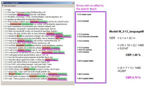
This means that even all the little mistakes are statistically full-fledged errors. Every missing comma, a “u” instead of a “v”, an additional space or even an uppercase letter instead of a lowercase letter are included in the CER as “whole errors”. The small details neither disturb the reading and understanding of the text nor do they prevent the search engine from finding a term.
So don’t only look at the numbers but also at the text comparison.Your model is usually better than the CER (and especially the WER) suggest.
To illustrate this, we have calculated this exemplary: